Operations research: a robotic job-shop cell

What it is

Five robotic arms at the project’s peak, conveyors, six part types, and a release order to decide for every batch.

What was hard

The plan has to drive arms that actually move, on a batch the machine only discovers when it looks at it.

What it proves

The gain sits in the path each part takes, not in how long the operations run. That is the opposite of what the brief led you to expect.

A solo project, on real hardware, within the operations research block of the engineering programme. 5weeksproductionFive weeks of work, alone from start to finish, from the camera to driving the arms., supervised through periodic progress reviews. Assessed by demonstration on a randomly arranged batch: the cycle ran to completion.

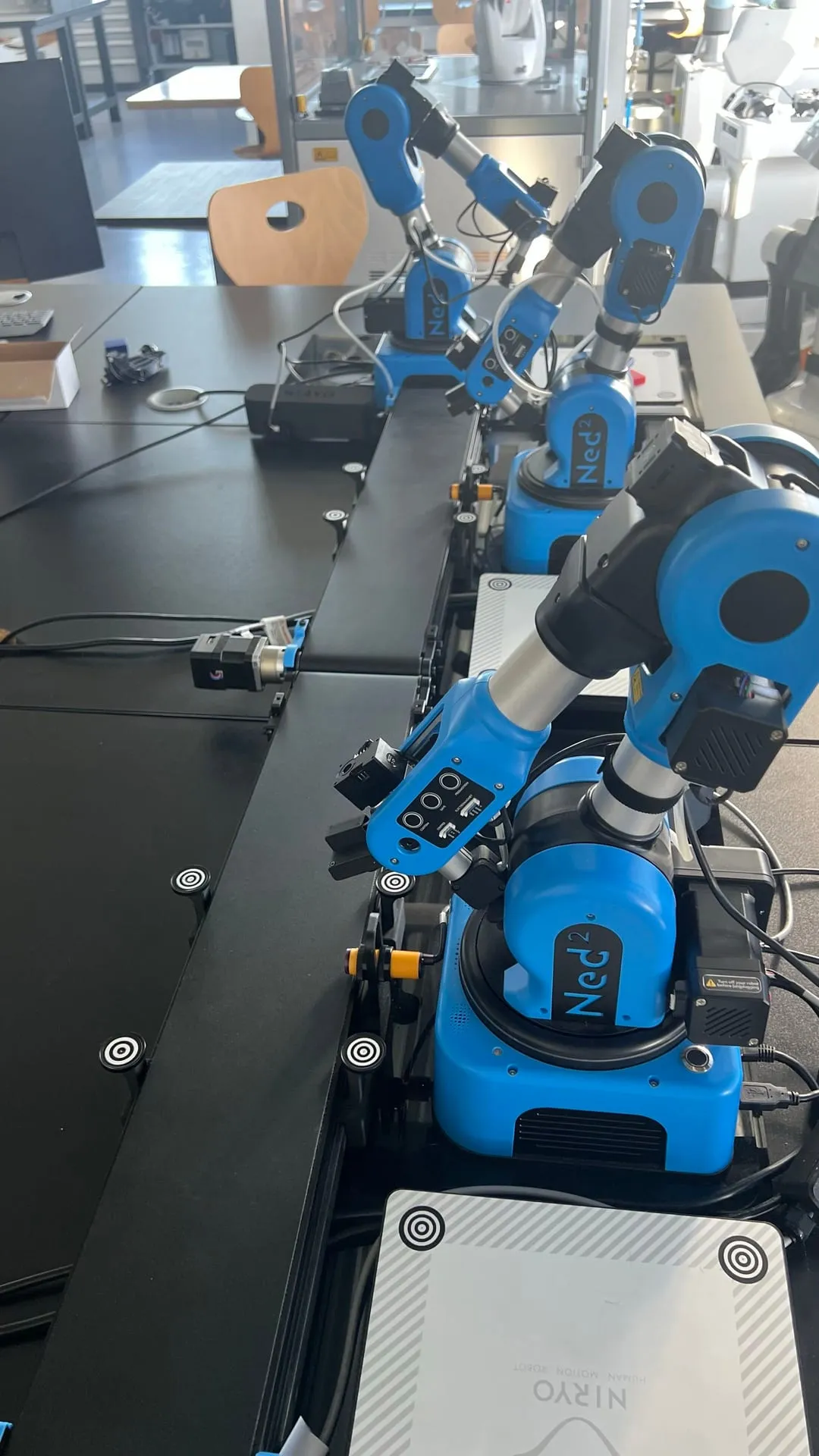
For four weeks I drove 5armsproductionFive real robots, each with its own job, and one piece of software moving the parts without collisions, from detection to drop-off. in parallel, each with its own program, positions, sequence and machining step: a whole miniature production line, from spotting the parts to the final drop-off. The measurements replayed below cover the configuration delivered at the end of the project, where three of those arms were still in service.

A cell that discovers its batch

A miniature production cell. Robotic arms linked by conveyors, a bin of parts at the start, two processing stations. The batch mixes 6part typesproductionTwo shapes times three colours: six different parts the camera tells apart on its own before deciding what to do with each.: two shapes crossed with three colours, each with its own machining time, and they do not all pass through the same stations.

The question is a textbook scheduling problem as stated: in what order should parts be released so the whole batch finishes as early as possible?

Nothing is declared, everything is seen

The workload changes every cycle. Which stations a given part type passes through is drawn at random when the batch starts. A part may go through both stations, one, or neither. The scheduler therefore never solves the same problem twice, and has to adapt to an instance it discovers.

The batch is not declared, it is seen. Nothing is keyed in: one arm observes the bin, and vision counts parts by shape and colour. What the system believes is on the belt is the output of a detection, with everything that implies about sensitivity to lighting.

Everything is distributed and asynchronous. Each arm is an independent process sharing no memory with the others. They coordinate by messages, and each must stay correct if a neighbour lags, restarts, or misses a pick.

Arms talking to each other

Robotic cell and scheduler

One line: the part travels past every arm

1. The bin of parts

   laid out at random, nothing is keyed in

2. the source arm moves in and photographs

   Vision

   counts the parts by shape and by colour

   six possible types

3. the list of parts in the batch

   Scheduler

   works out the order to release the parts

   The stations to visit are drawn at random

   per part type, on every batch: the problem changes each cycle

4. the running order

   Source arm

   releases the parts onto the conveyor, one at a time, in that order

5. the conveyor carries the part past arm 2

   Arm 2

   machines it, or lets it through

   Each arm either acts, or does nothing

   the part travels past all four arms in order

   it may be machined by one, by several, or by none

6. the conveyor carries on

   Arm 3

   machines it, or lets it through

7. the conveyor carries on

   Arm 4

   machines it, or lets it through

8. the conveyor carries on

   Arm 5

   machines it, or lets it through

9. end of the line

   Batch exit

   Observed times feed back to the scheduler

   transit and machining times measured, smoothed, reused on the next batch

A single node, parameterised by identity. The same program runs on every arm; its role, its neighbours, its positions and its workspace are derived from its identifier at startup. Adding a station does not mean writing a new program.

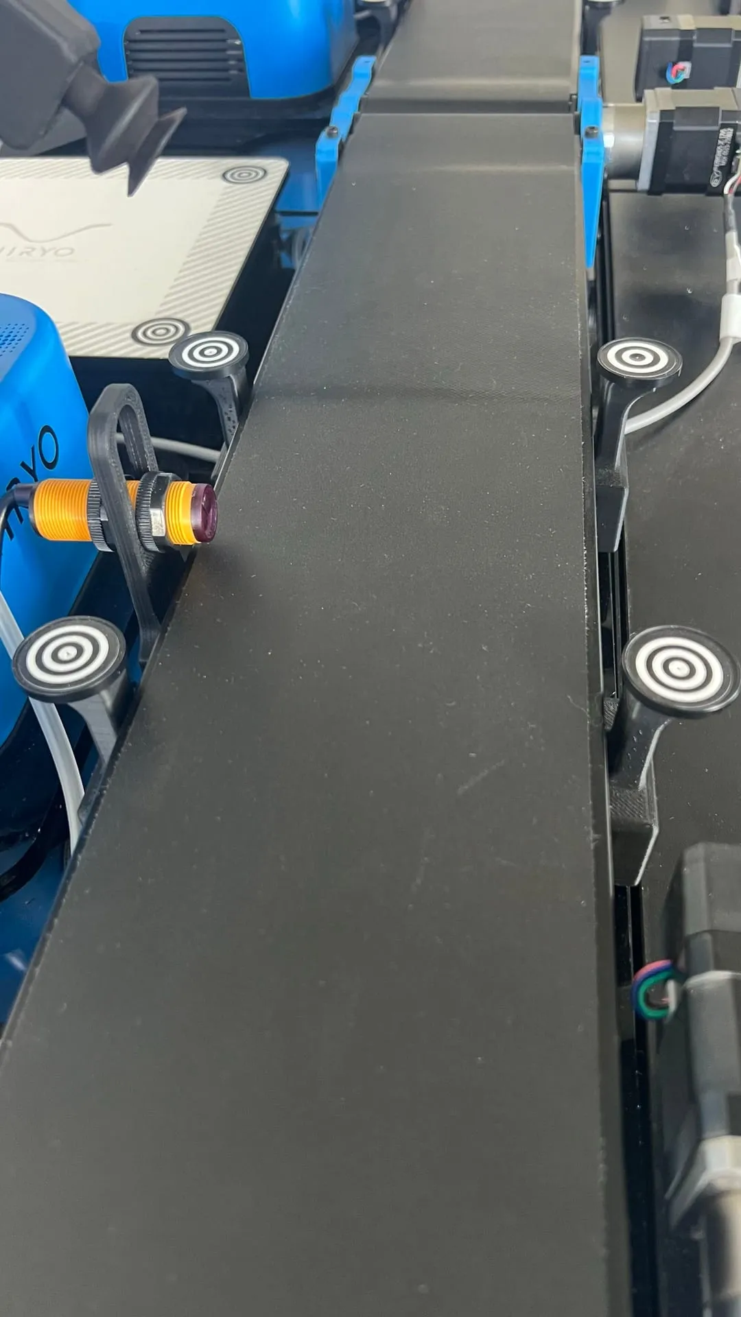
A publish-subscribe messaging layer carries commands, states, pick requests and the global emergency stop. Each node publishes a last will: if its process dies, the others see it go offline without waiting for a guard timeout.

A scheduling module separate from the control logic. It knows nothing of arms, conveyors or cameras. It receives a list of tasks and transit times, and returns an order. That separation is what made it possible, much later, to replay it entirely outside the cell: without it, none of what follows would have been measurable.

A metrics loop times the observed service and transit durations and smooths them continuously, so that the next plan rests on how the line actually behaves rather than on fixed values.

reproducible artefact

A real distributed cell: arms coordinated by messaging, vision-based detection, passage sensors, conveyors, and recovery from failed picks.

Giving up theoretical refinement

Admission by availability rather than by time slot. The plan computes, for each part, the ideal moment to release it, the one that makes it arrive just as the next station frees up. The protocol actually used ignores it: an arm asks, the station accepts if it is free, otherwise it declines and the request is retried.

This is a deliberate surrender of theoretical refinement, and it comes from a property of the shop floor: on a failed pick, a misdetected part or a slipping conveyor, a reserved slot becomes wrong immediately, and the whole downstream plan with it. Observed availability, by contrast, stays true by construction. I preferred a protocol that never lies to one that optimises for as long as nothing goes wrong.

Smoothing observed times instead of freezing them. Service and transit times are re-estimated continuously from what the line actually does. The price is described below: the smoothing starts from values set by hand, and the mechanism keeps no record of the observations.

Manufacturing the difficulty rather than waiting for it. Drawing the stations traversed at each cycle is deliberate: without it, one batch resembles the last and the scheduler has nothing to do. That choice is what made the problem exist, and, as we will see, it is also what carries the entire gain.

documented trade-off

Admission by availability rather than by time window: a station accepts a part when it is free, without negotiating a slot.

constraint met

Variable workload imposed at every cycle: the stations traversed are drawn at random per part type, which changes the problem instance from one cycle to the next.

What the scheduling returns

The cell works end to end. That is not the result worth publishing: a line that runs is an entry condition, not a conclusion. The result is what the scheduling module gives when you replay it.

Everything that follows is simulated. The module runs without hardware, and depends only on its configuration and the timings file. So I ran it as it is, outside the cell, on workloads drawn the way the real cycle draws them, comparing each strategy against the exact optimum obtained by enumerating the 720possible orderingssimulationPermutations of a full batch: 720 possible orderings (simulation). of a full batch. These numbers compare strategies against one another under a common model. None of them is a time measured on the line.

A fast method is enough, exhaustive enumeration buys nothing. Trying every possible order guarantees the best one, but their number explodes with batch size. A fast method still finds that same order 798out of 798 batches testedsimulationTo organise a production run you can try every possible order and keep the best, but the number of orders explodes with batch size. A fast method here gives exactly the same answer as the exhaustive search, on every single case tested., losing nothing along the way. Yet the scheduler switches to full enumeration as soon as the batch is small, precisely to guarantee that optimum: it pays a computation cost that explodes for a result it already had.

One of the strategies made available to the operator is harmful. The interface offers three methods. One of them, presented as a heuristic suited to job-shop problems, finishes 54.43% extra timesimulationTime lost by the strategy the interface recommended: 54.43 % extra time (simulation, n = 798). at the median and reaches the optimum on 0draws out of 798simulationDraws where the hybrid strategy reaches the optimum: 0 draws out of 798 (simulation, n = 798).. That is worse than not scheduling at all: releasing parts in the order they happen to arrive costs 17.13% above the exact optimumsimulationMedian gap of arrival order to the optimum: 17.13 % above the exact optimum (simulation, n = 798). at the median. Nobody could have known, because nothing ever compared two methods.

The lever is not where the brief assumed it was. The brief points towards processing durations: different parts, different times, an order to find. Yet varying those durations changes only 0.68%simulationUnder one percent: this was the lead the brief pointed at, and it returns almost nothing. Sixty times less than the parts' route.. Varying the route the parts take changes 40.23%simulationOn the same batch, the worst release order takes forty percent longer than the best. That is the gap the scheduling goes after., and up to 245.09%simulationLargest room for optimisation observed: 245.09 % (simulation, n = 1500). in the worst case. Sixty times more.

The reason is measurable: a station spends 93.2% of the timesimulationOut of a hundred seconds a station is busy, more than ninety are picking, moving and placing. Speeding up the machining cannot change the total time: what has to be optimised is the route the parts take. handling the part rather than machining it. Speeding up the machining therefore cannot move the total time. What moves it is unbalancing the two stations, and that is what the parts’ route does.

measurement

Simulated comparison of the scheduling strategies against the exact optimum, reproducible without hardware.

The displayed figure that means nothing

The total time announced to the operator does not depend on the computed order. At the end of planning, the cycle displays an estimated time alongside the name of the chosen method. That number is obtained by summing per-part contributions into two accumulators, and addition is commutative. Recomputed across the 720possible orderingssimulationPermutations of a full batch: 720 possible orderings (simulation). of a full batch, it takes 1valuesimulationDistinct values of the displayed makespan across all permutations: 1 value (simulation).. Whichever method is chosen, the screen shows the same number. The impossibility is structural.

The actual elapsed time was measured, but not kept. The line does time the batch’s actual duration and displays it at the end of the cycle, but nothing writes it down: no log, no file. That is the difference between not having measured and having measured without keeping the result, and the second is what applies here.

The service times are not measurements in the strict sense. The file holding them is the result of a smoothing started from values set by hand. It records no sample size, no date, no dispersion, and there is no way today to know how many observations went into it. All the simulations on this page inherit that: they are consistent with one another, not calibrated against reality.

The workload draw is not reproducible. It uses the clock as its seed, whereas the experimental function written for the same purpose accepts an explicit seed. Two cycles therefore cannot be replayed identically, which is exactly what would have been needed to compare two strategies on the line rather than in simulation.

There is no machining. Stations wait for a programmed duration. The per-type times are chosen constants, not physical properties.

Nothing is testable without the hardware. Every script in the test folder opens a connection to an arm: these are commissioning tools, not tests. There is no automated assertion anywhere, even though the scheduling module, the one carrying all the interesting logic, was perfectly testable offline, as this page demonstrates.

If I started over

I would make a number that cannot be right fail loudly. The time shown to the operator does not depend on the order, and nobody saw it, starting with me, for the whole project. Not through carelessness: because the number was plausible. It had the right order of magnitude, it changed when the batch changed, it carried the method’s name. Nothing in its appearance signalled that it was indifferent to the one thing it claimed to evaluate.

That is the worst kind of defect, because it breaks nothing: a crash gets noticed, a wrong but credible number settles in. The remedy is not to proofread harder, it is to make the error impossible to ignore. Here, an assertion comparing the announced time across two different orders of the same batch and refusing to start if they match. Three lines, runnable without a robot, and the defect would have surfaced on day one.

I would establish the floor before the optimum. The project built exhaustive search before checking that a heuristic would not do, and never compared its scheduling against no scheduling at all. The two controls, doing nothing and doing the simplest possible thing, cost half a day and would have answered the central question: is any of this worth it? They would also have surfaced the harmful strategy far sooner.

I would keep what I measure. One line written at the end of each cycle (batch, method, estimated time, actual time) and the project would today hold a comparison of estimate against reality across every run, instead of a memory. It was the missing measurement, and it was already being computed.